Practical 3-3: Stochastic birth-death model
Overview
In this practical you will see how we can make the code for the stochastic birth-death model safer, simpler, and more reusable.
Background
When running stochastic simulations we often want to run multiple simulations and compare outputs easily. In this practical we will learn how to efficiently plot multiple outputs on the same graph, and use a new set of functions contained within the SBOHVM/RPiR package on GitHub.
Tasks
In the previous practical your script repeated a section of code to
overlay multiple outputs on the same plot. We recommended that you use a
for loop to solve this problem, since copying and
pasting identical code is bad practice and can easily introduce
mistakes. In this practical, we’re going to attempt to improve our code
further by separating the simulation functionality from the model more
cleanly.
Look at run_simple()
Take a look at the new function run_simple() online. Go
to https://github.com/SBOHVM/RPiR, open on the R folder, and find the file called run_simple.R. It should look something
like this:
#' @title Simplest code to run a simulation loop
#'
#' @description
#' A generic function to run a simulation loop for a fixed period of time.
#'
#' @param step_function Function to run a timestep (step_function())
#' which returns a list containing elements updated.pop} with the
#' updated population and end.experiment which is TRUE if
#' the experiment has ended (FALSE if not)
#' @param initial.pop Initial population data frame with columns corresponding
#' to function requirements
#' @param end.time End of time simulation
#' @param ... (optional) any other arguments for step_function(), e.g.
#' parameters or timestep
#'
#' @return Data frame containing population history of simulation over time
run_simple <- function(step_function,
                       initial.pop,
                       end.time,
                       ...) {
  # Check whether step_function uses global variables
  if (length(findGlobals(step_function, merge = FALSE)$variables) > 0)
    warning(paste("Function provided uses global variable(s):",
                  paste(findGlobals(step_function, merge = FALSE)$variables,
                        collapse = ", ")))
  population.df <- latest.df <- initial.pop
  keep.going <- (latest.df$time < end.time)
  while (keep.going) {
    data <- step_function(latest.df, ...)
    latest.df <- data$updated.pop
    population.df <- rbind(population.df, latest.df)
    keep.going <- (latest.df$time < end.time) && (!data$end.experiment)
  }
  row.names(population.df) <- NULL
  population.df
}
The purpose of this new function is to separate out the simulation
functionality from the model, and to simplify and automate the running
of multiple stochastic simulations. If you look closely you can see that
the function run_simple() does the job we described in the
previous practical. It is set up in terms of the generically named
step_function argument, which in the case of the current
model would be the timestep_stochastic_birth_death()
function. Note however, that step_function requires the
function name without brackets since here we are passing the function
itself, rather than calling it:
final.populations <- run_simple(timestep_stochastic_birth_death,
                                initial.populations,
                                end.time,
                                birth.rate = some.specific.birth.rate,
                                death.rate = some.specific.death.rate,
                                timestep = short.timestep)
There are two things going on here that we haven’t seen before: (1)
We’re passing the step function as an argument to the
run_simple() function. This just happens like any other
argument being passed, you pass in the function, it gets assigned to the
step_function argument – remember that we can call it
anything inside a function – and then step_function gets
used just like initial.pop and all of the other arguments.
(2) the argument .... This is a way of saying “and there
will be other arguments I don’t want to (or can’t) specify”. You will
find this in lots of R code (see ?plot for example). For
us, the point is that each step function will need different
parameters passed to it, and we don’t know what they are in
advance. Instead we just pass them through:
data <- step_function(initial.pop, ...)Any arguments after the three fixed arguments of
run_simple()must be named – since they will be blindly passed straight through to the step function (via the...).
Write a demo
Now write a new demo called d0303_run_birth_death using
run_simple() to replace the whole simulation loop in the
earlier code. This should make the code in d0302_stochastic_birth_death more
compact, and will also make it much less prone to error, as we’ve
isolated 10 more lines of code that we never need to write (or copy and
paste) again.
If you encounter any problems, RPiR has a function,
run_simulation(), that does some additional checking and
reporting if you set an additional argument debug = TRUE,
which may help you identify what’s going wrong. We’ve mostly suggested
using run_simple() here as it’s significantly easier to
follow what’s going on in the function, but in future exercises, it’s
better to use run_simulation() for everything as it has
some other additional functionality.
Report
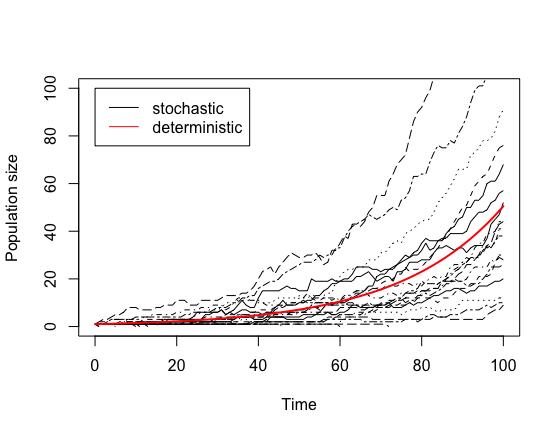
1. Compare stochastic and deterministic models
Run the stochastic birth death model with a birth rate of 0.06, a
death rate of 0.02, an initial population count of 1, and a timestep of
1. Observe the variability in the outputs. Overlay the deterministic
model results on the same plot. Note that you can’t use the
run_simple() or run_simulation() function with
the old step_deterministic_birth_death() step function
because it doesn’t know about the time column in the data
frame or timesteps, so you just need to copy the for ()
loop from the d0105... demo to get the deterministic
result. You should get something like this:
plot
2. Increase the initial population size
What happens to the variability as you increase the initial
population size? You may want to adjust the scale of the y-axis to see
what happens at larger population sizes. To automate this, you can set
the y-axis upper limit to \(100
\times\) initial.count by setting
ylim = c(0, 100 * initial.count). Report these results in
your demo.
Check it works
As with previous exercises, you need to check that everything works correctly – that the package installs, and the demos and help files work and you can generate reports from the demos – and then we want you to get a couple of other people in your subgroup to check your code and make sure it works for them, and we want you to check other people’s code too. We describe how to do this for packages in GitHub in Practical 3-1 (also under Check it works) if you’re uncertain.
Remember, interacting like this through GitHub to help each other will count as most of your engagement marks for the course.