Practical 3-2: First stochastic birth-death model

Overview

In this practical we will run our first stochastic simulations, starting with the stochastic version of the birth-death model. From now on, we will expect a brief report in some format on every practical, so we will not give explicit guidance in every case.

Background

In the lecture, we discussed the fact that the deterministic models we have been using so far don’t handle dynamics at the individual level well. To capture individual-level behaviour we need to include an element of chance in the model. This new type of model, which includes a probabilistic element, is called a stochastic model.

Tasks

To write a model to handle stochastic population dynamics we obviously have to update the timestep function to handle the new dynamics. However, we also have to understand whether anything else has changed in how the simulation works. In fact, something has. There is now the chance that the population will die out before the end of the experiment, so we need to look for this happening – not least to speed up the simulation.

1. Write a demo

We’ll start by writing the structural code in a new demo file. In Practical 3-1 we created this file and named it demo/d0302_stochastic_birth_death.R. Currently, the demo is a copy of the d0105_run_birth_death demo, which is a good starting point. In this Practical you will edit this code.

From Practicals 2-3 and 2-4 we have a while() loop which runs the simulation, e.g.

while (latest.population$time < end.time) {
  latest.population <- timestep_deterministic_SIS(latest.population, 
                                                  ecoli.transmission, 
                                                  ecoli.recovery, 
                                                  timestep)
  population.df <- rbind(population.df, latest.population)
}

The loop ends when the time runs out. Now, instead, there are two reasons why we might stop the simulation – the time may have run out, or the timestep code may identify that the dynamics are now complete. To achieve this, the timestep code will have to return both the updated population and whether the simulation is over. We suggest doing something like this:

while (keep.going) {
  data <- timestep_stochastic_birth_death(latest.population, 
                                          human.annual.birth, 
                                          human.annual.death, 
                                          timestep)
  latest.population <- data$updated.pop
  population.df <- rbind(population.df, latest.population)
  # The experiment may end stochastically or the time may run out 
  keep.going <- (!data$end.experiment) && (latest.population$time < end.time)
}

We’re going to have to change the function timestep_stochastic_birth_death shortly so it returns this additional information.

Notice also that at the start of the loop keep.going has not yet been defined, which will cause an error, so you will need to start it off with an appropriate value.

Remember that library(RPiR) at the top of the script loads plot_populations(), and library(githubusernameSeries03) loads timestep_stochastic_birth_death(), which means you no longer need to source any helper files.

2. Write a function

You will need to write the timestep_stochastic_birth_death() function to provide the right information to the main loop. We created this file in Practical 3-1, but the function itself contains the deterministic step function for single species population dynamics, step_deterministic_birth_death() (from Practical 1-5). This is a useful starting point. Starting with this code, you need to make three changes.

First, we need to handle the effect of changing timesteps and update the code with something like this:

timestep_stochastic_birth_death <- function(latest, 
                                            birth.rate, 
                                            death.rate, 
                                            timestep) {
  # Multiply birth and death rates by timestep
  effective.birth.rate <- birth.rate * timestep
  effective.death.rate <- ____ * ____
  
  # Determine the numbers of new births and deaths
  
  
  # Store new time and count in a dataframe
  next.population <- data.frame(time = latest$time + timestep, 
                                ____ = ____)
  
  # Determine whether the experiment is finished
  
  
  # Return both of these pieces of information
  
  
}

Then we need to make the simulation stochastic using rbinom(). Remember, if you want to draw once from the binomial distribution with count trials, and a probability of success of prob, then the number of successes is:

new.events <- rbinom(1, count, prob)

So, the key is to use the rbinom() function to determine the numbers of new births and deaths in each time step. The number of births is drawn from a binomial distribution with size count and probability birth.rate * timestep, and the number of deaths is drawn from the same distribution with probability death.rate * timestep.

We then store the next timestep and next count values in a dataframe.

Then we need to determine whether the experiment is finished. In this case, the experiment will only end if the population completely dies out, so:

is.finished <- (____ == 0)

You just need to work out what the blank should be…

Finally, we need to return both the updated population and simulation state (whether the simulation has ended) from the function. Since a function can only return one item, we will have to return a list with two elements at the end of the function:

list(updated.pop = next.population, end.experiment = is.finished)

Note that the rbinom() function is in the stats library, so you could perhaps more correctly call it as stats::rbinom(1, count, prob), and then add the stats library to your package’s dependencies by typing usethis::use_package("stats") in the console (this will update the DESCRIPTION file). Finally in the R/githubusernameSeries03-package.R file, you need to import the functions from this library, as you already have for RPiR:

#' @import RPiR
#' @import stats

Doing this is not strictly necessary since stats is a core built-in R library, but it will be necessary if you use any functions from other libraries in later exercises. We described this for RPiR in Practical 3-1 in the Package metadata and dependencies section.

You can determine what library a new function you use is in if you’re not sure by looking at the top left hand corner of the help file for the function – here it says Binomial {stats}, the library name is in curly brackets. If it says {base}, that means it really is built in to R and doesn’t need qualifying like this.

Once you’re happy with your function, run devtools::document() to generate man/ files and edit the NAMESPACE. Then run devtools::install() to permanently install it.

Report

When you are happy that the code is working and makes sense, start working on your report (in your demo/d0302_stochastic_birth_death.R demo file). Remember that you can run your code by

compiling a notebook, or by
running it as a demo

demo("d0302_stochastic_birth_death", package = "githubusernameSeries03")

1. Demonstrate stochasticity

Run the code several times with a birth rate of 0.2, a death rate of 0.1, an initial population count of 1, and a timestep of 1. Since we’re repeating the piece of code doing the simulation, you could do this using a for loop. The stochasticity means that we see variable outputs. This is most easily demonstrated if you plot multiple results in the same figure, which you can do with an if statement. You should get something like this:

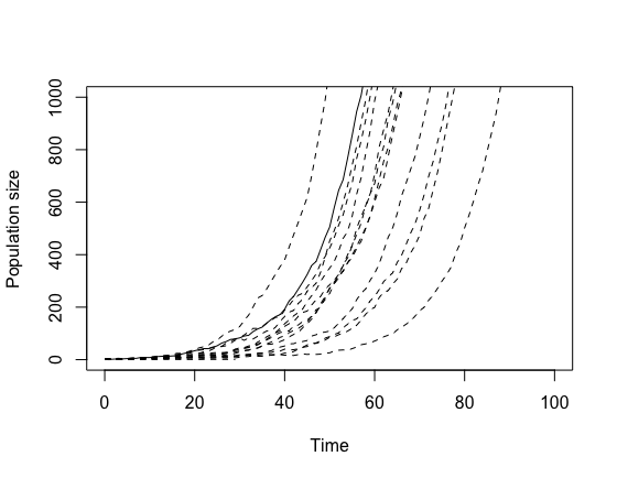
plot

2. Increase variability

Increase birth and death rates or the time you’re simulating over to increase visible variability. Again, you could use a for loop to generate outputs over a range of different rates / time periods.

3. Increase timestep

If you haven’t already, try increasing the value of timestep. What happens? You are actually getting impossible numbers (NAs) because the probability of giving birth has got above 1. You can fix this by using the stop() command inside your timestep_stochastic_birth_death() function to stop running code when the numbers you put in are impossible:

if ((effective.birth.rate >= 1) || (effective.death.rate >= 1))
  stop("Effective rate too high, timestep must be too big")

Remember that for this stop() command to be effective you have to put the test after you define the variables you are checking, but before you use them! Rerun the code and check it stops when appropriate.

Check it works

As with previous exercises, you need to check that everything works correctly – that the package installs, and the demos and help files work and you can generate reports from the demos – and then we want you to get a couple of other people in your subgroup to check your code and make sure it works for them, and we want you to check other people’s code too. We describe how to do this for packages in GitHub in Practical 3-1 (also under Check it works) if you’re uncertain.

Remember, interacting like this through GitHub to help each other will count as most of your engagement marks for the course.