Reproducible Programming
What do you want to do?
- Access data
- Build models
- Test hypotheses
- Run analyses
- Report the results
- Share the results and the techniques with others
What’s different about R?
What’s different about R?
- Formulae and factors
- Data frames
- Subsetting data
- Plotting data and generating reports and saving them to disk
- Massive database of user-supplied packages
- Specialised Integrated Development Environment (IDE)
- RStudio
- Trivial to create your own packages
- Integration with GitHub
What are formulae?
- Formulae!
- Compact symbolic form for storing formulae for model building
?formula
What are factors?
- Vectors
- but for data in a fixed number of categories, possibly ordered
- Compact form for storing categorical data for model building
?factor
?ordered
?levels
What are data frames?
- Tables (as from a spreadsheet)
- One or more rows of data
- Named columns of fixed type
- Fundamental data structure for most modelling functions
head(mtcars)
##                    mpg cyl disp  hp drat    wt  qsec vs am gear carb
## Mazda RX4         21.0   6  160 110 3.90 2.620 16.46  0  1    4    4
## Mazda RX4 Wag     21.0   6  160 110 3.90 2.875 17.02  0  1    4    4
## Datsun 710        22.8   4  108  93 3.85 2.320 18.61  1  1    4    1
## Hornet 4 Drive    21.4   6  258 110 3.08 3.215 19.44  1  0    3    1
## Hornet Sportabout 18.7   8  360 175 3.15 3.440 17.02  0  0    3    2
## Valiant           18.1   6  225 105 2.76 3.460 20.22  1  0    3    1
?data.frame
?read.csv
?read.table
How do we subset vectors?
vec <- c(1, 2, 3)
vec[vec > 2]
## [1] 3
vec <- 1:3
vec > 2
## [1] FALSE FALSE TRUE
vec <- seq(from = 1, to = 3)
subs <- c(T, F, T)
vec[subs]
## [1] 1 3
How do we subset data frames?
df <- data.frame(val = c(1, 2, 3),
                 other = c("a", "b", "a"))
df$other
## [1] "a" "b" "a"
df[df$other == "b", ]
##   val other
## 2   2     b
subset(df, val == 1)
##   val other
## 1   1     a
How do we subset data frames?
But these things are constantly evolving:
library(dplyr)
df %>% filter(other == "b")
##   val other
## 1   2     b
mtcars %>% filter(mpg > 20) %>% filter(carb >= 4)
##               mpg cyl disp  hp drat    wt  qsec vs am gear carb
## Mazda RX4      21   6  160 110  3.9 2.620 16.46  0  1    4    4
## Mazda RX4 Wag  21   6  160 110  3.9 2.875 17.02  0  1    4    4
How do we plot?
plot(c(1, 2, 3), c(1, 2, 1))
lines(c(1, 2, 3), c(2, 1, 2))

How do we plot?
Again, there are much more sophisticated ways, as you know… e.g.
library(ggplot2)
mtcars %>% ggplot(aes(wt, mpg)) + geom_point() + geom_smooth()

How do we save to disk?
png("out.png")
plot(c(1, 2, 3), c(1, 2, 1), type = "l")
dev.off()
?pdf
?png
?Devices
How do we save to disk?
Again, using ggplot2…
g <- mtcars %>% ggplot(aes(wt, mpg)) + geom_point() + geom_smooth()
ggsave("out.png", g)
?ggsave
How do we use packages?
Install it first:
install.packages(c("tibble"))
or from RStudio menus, and then use it:
library(tibble)
not forgetting:
update.packages()
occasionally.
So how do you learn to program?

What do you want to do?
- Access data
- Build models
- Test hypotheses
- Run analyses
- Report the results
- Share the results and the techniques with others
What are you going to do?
Learn how to:
- Write code
- Write documentation
- So you can come back and understand it later
- Identify and isolate reusable code
- So you don’t have to write it again later
- Generate documented results
- Read and understand other people’s code
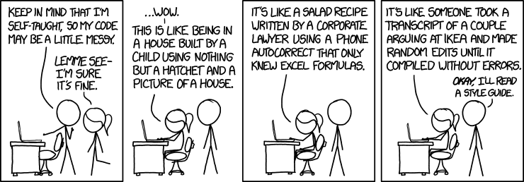
Remember…

“I honestly didn’t think you could even USE emoji in variable names. Or that there were so many different crying ones.”
What are you going to do?
- Read and write well-documented and well-structured code
- Use this to generate clear and well-documented results/reports
How are you going to do it?
- Problems will be structured around population dynamics, epidemiology and biodiversity
- They will start off easy and ramp up
- Packages (libraries) will allow you to solve many problems easily, but we are focusing on problems they don’t help with!
Have fun!

Starting with…
- Practical 1.1 - 1.6 (“practical1-x”) on population dynamics
and optionally:
- Practical A.1 - A.3 (“practicalA-x”) on if statements, functions and loops